Highlights
- Construction of gridded temperature sections and SSS data for each transect, as well as climatological monthly mean data and annual summer mean DJFM data of the surface salinity and upper ocean temperature near 140°E at high-resolution over the seasonal heating cycle (Oct to Mar). Distributed via SEDOO: XBT website https://doi.org/10.6096/11, TSG website: http://sss.sedoo.fr/. Used extensively for ocean model validation.
- Characterisation of the seasonal mixed layer property variations in relation to the surface ocean heat and freshwater budgets. (link to science result 1).
- Document the long-term temperature changes within different water-masses across our section over 25-years, and how the trend compares to the interannual variability (Auger et al., 2020). (link to science result 2). Three regions stand out as having strong change that is radically different from the interannual variability :
o (A) warming of the deep-reaching subantarctic waters (0.29±0.09 °C/dec) in the northern part of our section;
o (B) cooling of the near-surface subpolar waters close to Antarctica that extends down to 200 m depth (-0.07±0.04°C/dec), in a region of long-term cooling in SST
o (C) significant warming of the subsurface subpolar Circumpolar deep waters (0.04±0.01°C/dec), associated with a large shallowing (39±11 m/dec).
- Subsurface Winter Water layer temperatures undergo large interannual variations that overwhelm any long-term trend, and lagrangian tracking show they are correlated (r=0.68) with the SST of the previous winter located further upstream in the subpolar Australian-Antarctic basin (120-145°E; 57-61°S). (link to science result 3).
- The underway SSS data reveals the seasonal and interannual variations in the surface salinity, the critical variable for ocean stability in the Southern Ocean . (link to science result 4). In particular :
o Seasonal freshening of the surface Antarctic waters over the summer sea-ice melting cycle
o Interannual SSS variations in the north of the section are linked to input of Subtropical waters from the Tasman Sea, and cold eddies from the SAF
o Biannual SSS variations in the Antarctic Zone are linked to upstream sea-ice coverage and melt in the preceding spring
o Surface salinity and the freshwater budget close to Antarctica vary mainly in relation to seasonal sea-ice cover and melt, and not E-P, and were largely impacted by the Mertz glacier calving in 2011.
List of 4 science results and others:
Science result1: Seasonal variability of heat content across the Southern Ocean at 140°E
Our knowledge of heat content variability in the surface layer of the Southern Ocean has been greatly improved by SURVOSTRAL’s XBT observations. In the Subantarctic Zone, between the Subtropical Front and the Subantarctic Front, SURVOSTRAL XBT data have been used to better understand variations in the summer mixed layer, and temperature variations in the underlying winter layer (Trull et al., 2001; Rintoul and Trull, 2001; Chaigneau 2003; Chaigneau et al., 2004). The impact of these surface variations on the characteristics of sub-Antarctic modal waters was also analysed using SURVOSTRAL observations (Herraiz-Borreguero et al., 2010).
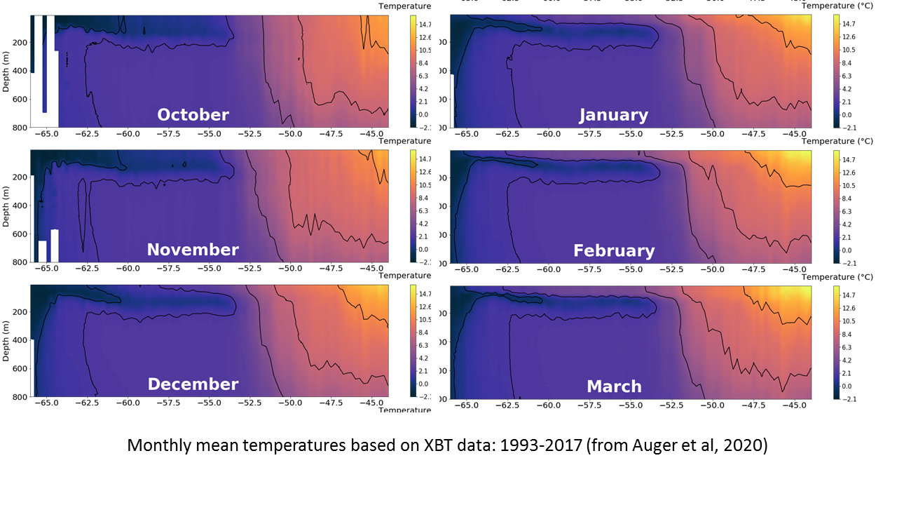
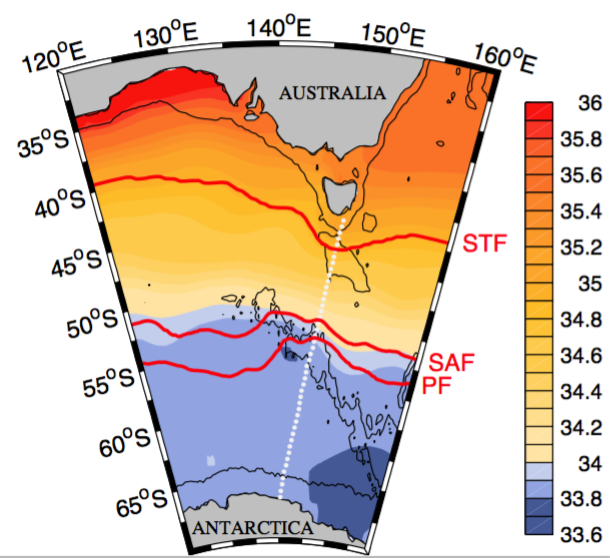
More recent analyses of the monthly mean temperature structure based on the 25-years of Survostral data by Auger et al. (2021) have revealed the stability of the seasonal cycle described by Chaigneau et al. (2004) based on only 8 years of data. The monthly mean temperature sections from October to March (Figure 1.1) calculated from the 25-year time series are quite similar to those calculated by Chaigneau et al. (2004). The water masses with the strongest seasonal changes are at the surface: the Antarctic Surface Waters (AASW) south of the Polar Front show the largest monthly mean variations over the summer warming cycle with coolest waters observed at the end of winter in late Oct-Nov. In the north of the section, there is a seasonal southward and deepening expansion of Subtropical waters throughout the summer season.
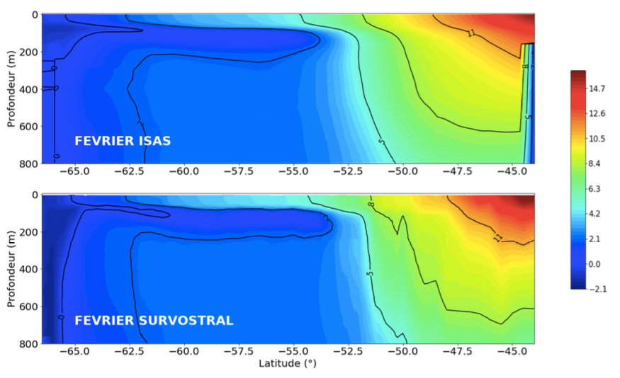
In 2004, comparisons with the Levitus T-S climatology in this pre-Argo era highlighted that the smoothing in the climatology was much too strong in this area, the seasonal cycle was poorly represented in surface salinity and in mixed layer depth (Chaigneau et al., 2004). Since 2005, there has been a large increase in the number of T/S profiles available from the Argo network over the upper 2 km, and daily and weekly gridded data sets are now available at 0.5° resolution, such as the ISAS/CORA gridded data from Coriolis (Cabanes et al., 2013). Although the ISAS gridded product includes the SURVOSTRAL XBT data, it is smoothed over 300 km in radius, which reduces the sharp frontal structures, compared to the Survostral gridded product with much less smoothing (0.5° resolution increasing to 0.25° resolution across the fronts from 49-54°S; Auger, 2019; Figure 1.2). Maintaining the highest resolution along the Survostral repeat transects is valuable for studying the fine-scale frontal processes.
Science result 2: Long-term trend in upper ocean temperature
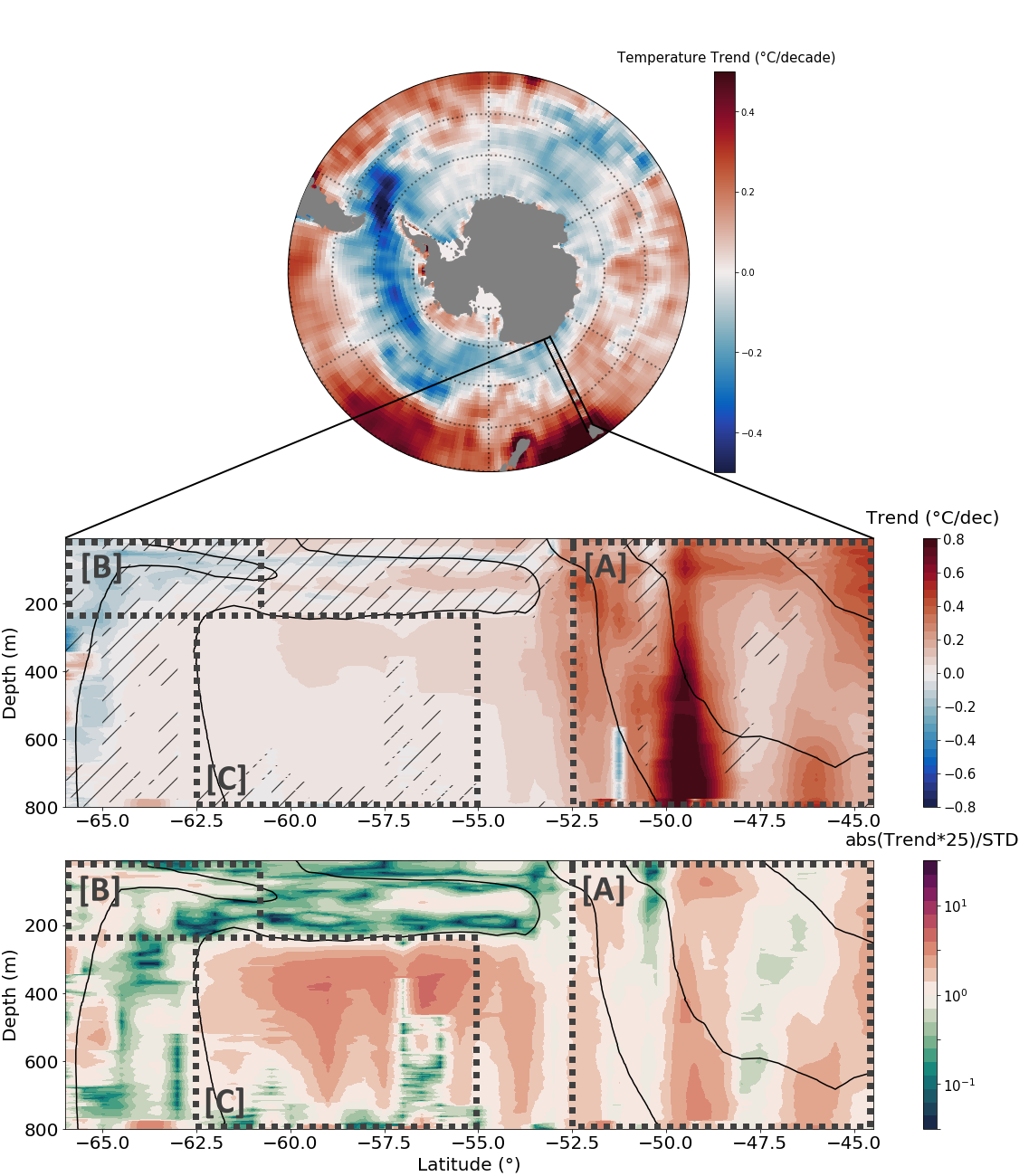
The 25-year Survostral time series has allowed us to better document the long-term temperature changes within different water-masses across our section, and how the temperature trend compares to the interannual variability (Auger et al., 2021). Three regions stand out as having strong change that is radically different from the interannual variability (Figure 2.1):
(A) warming of the deep-reaching subantarctic waters (0.29±0.09 °C/dec) in the northern part of our section, with similar values to those described by previous studies (Gille, 2008; Böning et al., 2008; Giglio and Johnson, 2017);
(B) cooling of the near-surface subpolar waters that extends down to 200 m depth (-0.07±0.04°C/dec), in a region where the long-term trend in SST also shows cooling over 25-year (Figure 5a), as described by Amour et al., (2016);
(C) significant warming of the subsurface subpolar deep waters (0.04±0.01°C/dec).
Our results highlight that this subsurface warming of subpolar circumpolar deep waters is, counter-intuitively, the most distinct change of the section with regard to interannual variability.
We observe larger warming in the upper part of the layer, which may be due to increased stratification at the base of the Winter Water layer due to surface freshening, that would reduce vertical mixing and heat removal from below (Marshall 2015, Armour et al. 2016). This robust warming of the circumpolar deep waters is associated with a large shallowing (39±11 m/dec), which has been significantly underestimated by a factor of 3 to 9 in past studies (Schmitdko et al., 2014). These Circumpolar Deep Water temperature changes are of comparable magnitude to those reported in West Antarctica (Rignot et al., 2019). This may have important consequences for warmer deep waters impinging onto the continental shelf downstream (Shen et al., 2018), with an impact for our understanding of future Antarctic ice-sheet mass loss.
These deep-reaching warming trends are associated with sea level rise, and the Southern Ocean south of Australia shows a fairly significant sea level rise during the 1990s (Lombard et al., 2006), and this increase is accelerating in the Southern Ocean in the last two decades (NASA). In an earlier study, Morrow et al. (2008) calculated the contribution of the deep-reaching temperature changes over the upper 800m from SURVOSTRAL data to the equivalent altimetric sea level variations here. A simple Sverdrup transport model showed how large-scale changes in the wind forcing, related to the Southern Annular Mode, may contribute to the deeper warming observed south of the SAF.
Science result 3: Interannual variability of temperature and heat content in the Southern Ocean
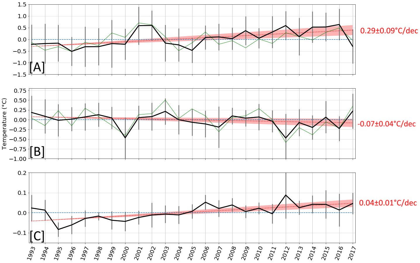
Auger et al (2021) identified the water masses across the SURVOSTRAL line where the interannual variability is strong, and dominates the trend (science result 2). Figure 3.1 shows the temporal evolution of the summer mean NDJF temperature anomalies over 25 years, for 3 key regions :
In zone (A) in the Subantarctic Zone, strong interannual variations exist in the heat and haline content (Sokolov and Rintoul, 2003; Morrow and Kestenare, 2014), linked to movements of the Subtropical Front. These variations also respond to changes in Mode Water volume in the area, modified by interannual variations in the input of warmer, saltier water from the Tasman Outflow – a southward extension of the East Australian Current. Altimetry tracking of eddies has allowed us to identify years when more warm-core eddies propagating from the north cross the Survostral line (2001, 2002, ..), or years when more cold-core eddies spawned from the SAF are observed by the XBT profiles (1994-1996) (Morrow et al., 2004; Morrow and Kestenare, 2014; Pilo et al., 2015). The large input of heat from the north in 2000-2001 follows the strong La Nina events in the southwest Pacific (Morrow and Kestenare, 2014; Pilo et al., 2015), and La Nina conditions are more prevalent over the last decade (2007-2017).
In zone (B) close to the Antarctic continent, there is a cooling trend in the upper 200 m with large interannual variations. The stronger interannual variability is evident in temperature, SSS and sea-ice, with cooler, low salinity waters in summer linked to larger sea-ice content in spring (Auger et al., 2021; Morrow and Kestenare, 2017). Lower temperatures from 2011 onwards are impacted by local coastal circulation changes and increased ice flow, following the Mertz Glacier calving just upstream. Morrow and Kestenare (2017) proposed that the cooling and freshening of the subpolar AASW waters near 140°E from 1999 onwards, may be impacted by meridional shifts of the zonal wind position and an associated change in the sea-ice cover.
The generalized warming trend of the Upper Circumpolar Deep Waters in zone (C) shows little interannual variation, being below the seasonal mixed layer.
Antarctic Surface Water and Winter Water interannual variability.
The Antarctic Surface Water (AASW) region from 53-62°S has strong interannual variability over the surface mixed layer and the Winter Water layer (Chaigneau et al., 2004; Auger et al., 2021);
In the core of the Winter Water layer, defined as the layer with temperature colder than 2°C between 55°S and 61.5°S, the temperature undergoes large interannual variations that overwhelm any long-term change, with peak-to peak temperature ranging from 0.92 to 1.28°C (Auger et al., 2021). These temperature variations within the Winter Water core along the Survostral line near 140°E are positively correlated (r=0.68) with the sea surface temperature of the previous winter further upstream in the subpolar Australian-Antarctic basin (120-145°E; 57-61°S), where the Winter Waters were modified at the surface (altimetric lagrangian backtracking was used to identify when the sub-surface winter water layer was last in contact with the atmosphere).
Science Result 4 : Sea surface salinity variations and the freshwater budget in the Southern Ocean.
Data from the SURVOSTRAL thermosalinograph enabled us to specify the seasonal structure of long-term surface temperature and salinity and to validate the climatologies in this region (Chaigneau and Morrow, 2002; Morrow and Kestenare, 2014). Early studies showed that the seasonal temperature cycle is well represented by the climatological data from Levitus, but the climatological salinity cycle is too smooth in the frontal regions, and too variable south of 50°S. These salinity biases are now corrected with the new salinity climatologies based on Argo data (eg ISAS/CORA from Coriolis), although the fronts remain too smoothed in these gridded products, and the coastal structure in the north and south of the sections as not well sampled by Argo data. SURVOSTRAL SSS products retain the highest spatial resolution across the ACC (Figure 4.1).
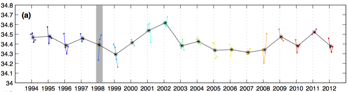
In the Subantarctic region north of the Subantarctic Front, interannual variations in the summer SSS and SST signatures (Figure 4.2) are linked to the latitudinal movements of the Subtropical Front (Morrow and Kestenare, 2014). When this front shifts southward, more high salinity subtropical waters are brought into the domain. Rather than responding to local wind stress forcing, the interannual SSS variability is strongly linked to southward flow from eastern Tasmania (the Tasman outflow), dominated by eddy movements (Pilo et al., 2015). A freshwater budget in the surface layer shows that variations in the local surface freshwater (P-E) forcing make a minor contribution to the SURVOSTRAL SSS signature. There appears to be a regime shift in the surface forcing and the SSS response, before and after the large perturbation in 2001–2002 following the 1999-2000 La Nina event.
In the Antarctic Zone south of the Polar Front, surface salinity observations from the SURVOSTRAL programme show that salinity at high latitude decreased by 0.1 during the period 1992-2004; this small decrease was initially linked to an increase in precipitation between 50-60°S during this period (Morrow et al., 2008). Recent analyses over a longer 20-year period covering 1992-2011, and with several products of evaporation and precipitation fluxes have revised this result. The decline in salinity was quite marked in the early 1990s, but since 2002, salinity in the Antarctic Zone has stabilized (Figure 4.3). The 20-year SSS trend is not significant (Morrow and Kestenare, 2014). The different freshwater flux products vary between them, and no product follows the observed salinity evolution.
Lateral advection is a key factor in these interannual variations in the Antarctic Zone (Morrow and Kestenare, 2014). Each year, the path followed by the waters detected along the SURVOSTRAL line varies, either with a direct path from the sea ice zone, or with a longer path further north where surface melt waters have more time to mix with saltier subsurface waters. Thus, the SSS response in the Antarctic Zone is more complex than originally estimated.
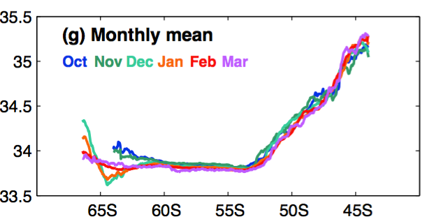
In the Sea Ice Zone (SIZ) south of 60°S, SSS shows distinct seasonal variations, based on 22-years of Survostral data (Morrow and Kestenare, 2017). In the northern sea-ice zone during the warming, melting cycle from October to March, waters warm by an average of 3.5 °C and become fresher by 0.1 to 0.25. In the southern sea-ice zone, the surface temperatures vary from − 1 to 1 °C over summer. The largest SSS range occurs in December, with a minimum SSS of 33.65 near the Southern Boundary of the ACC, reaching 34.4 in the shelf waters close to the coast. The main fronts, normally defined at subsurface, are shown to have more distinct seasonal characteristics in SSS than in SST.
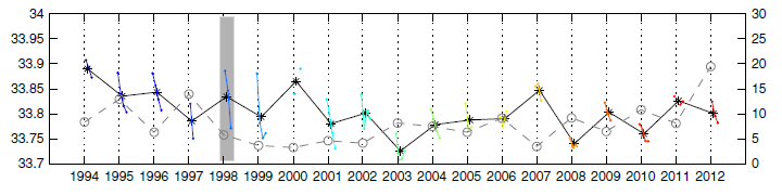
Interannual variations in SSS in the SIZ were more closely linked to variations in upstream sea-ice cover than surface forcing (Figure 4.4). SSS and sea-ice variations show distinct phases, with large biannual variations in the early 1990s, weaker variations in the 2000s and larger variations again from 2009 onwards. The calving of the Mertz Glacier Tongue in February 2010 led to increased sea-ice cover and widespread freshening of the surface layers from 2011 onwards. Summer freshening in the northern sea-ice zone is ~0.05–0.07 per decade, increasing to 0.08 per decade in the southern sea-ice zone, largely influenced by the Mertz Glacier calving event at the end of our time series. Knowledge of these interannual variations and trends is important because a large volume of fresh water in summer can create a barrier layer at the surface, thus limiting vertical exchanges between the cool, fresh surface waters and the warmer deeper layers, contributing to a net warming of the deeper water masses.
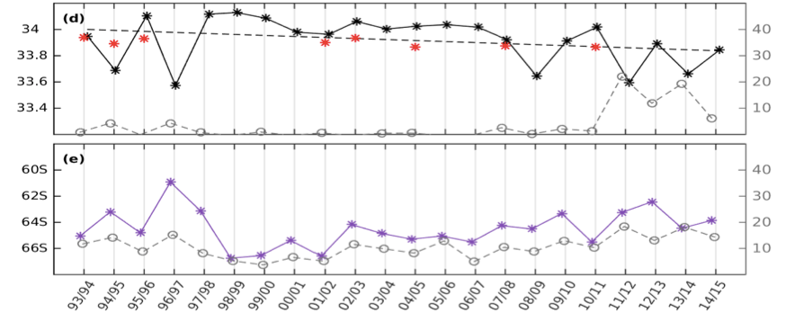
Bottom panel) November averaged latitudinal position of the zonal zero wind stress in the box 140-145°E (in violet), versus the December mean sea-ice coverage in the 135-140°E box (in grey). (Morrow & Kestenare, 2017).
Other studies
Survostral XBT and TSG data have been used in a wide range of scientific studies. A short selection is include here :
- The variability of baroclinic transport across the ACC has been estimated from a combination of SR3 CTD measurements, relative to 2500m, and the temperature in the surface layer measured from Survostral XBTs. The variability of this baroclinic transport (relative to 2500m) is estimated at ~8 Sv from SURVOSTRAL data (Rintoul and Sokolov, 2001), compared to the mean transport of 147 ± 10 Sv across the SR3 section.
- The time series of barotropic transport across the ACC has been estimated from XBTs, SR3 CTDs and satellite altimetry from 1992 onwards, based on the strong correlation between steric height variations and barotropic transport variability (Rintoul et al., 2002).
- The time-variable position of ACC fronts has been estimated using absolute dynamic height contours from satellite altimetry. This technique can follow 3 fronts over 25 years (SAF-N, SAF-S, PF; Sallee et al., 2008) distributed online (ctoh.legos.obs-mip.fr/data/datasets/Polar_Fronts) or up to 10 ACC fronts (Sokolov and Rintoul, 2003). The tuning of these algorithms was validated in using SURVOSTRAL XBT data (Sallee et al., 2008; Auger, 2019).
- Dynamic processes that generate deep jet instability in the CCA, were investigated using a combination of modeling, altimetric analysis and SURVOSTRAL XBT sections. Chapman and Morrow (2013) revealed that jets can « jump » between different bathymetric fracture zones. A vortex dipole develops on either side of the jets, and the variability in the dipole amplitude is well correlated with the frequencies of « jumping ».
- Improving the spatial resolution of hydrological fronts, via the lateral advection provided by altimetry. Altimetric currents horizontally stirred daily maps of low-resolution, gridded 2D T and S fields based on ISAS/CORA data in the Southern Ocean over a period of 7-15 days (Dencausse et al., 2013). This lateral advection generates a cascade of energy towards the smaller scales, which can create more turbulent and intense fronts. SURVOSTRAL high-resolution SSS and XBT measurements, with very fine-scale resolution of polar fronts, were used to validate this technique in this region of the Southern Ocean, and to derive the optimal duration of advection.
- Lagrangian pathways of interocean exchange. SURVOSTRAL XBT sections and SR3 CTD sections have been used to validate numerical models investigating inter-ocean exchange south of Tasmania. Southern Ocean mode and intermediate waters have been tracked using numerical models starting from the 140°E section into the Indian Ocean (Koch-Larrouy et al., 2009) and into the Pacific Ocean (Hasson et al., 2011); the critical starting point of these models were validated with Survostral data.
- Mode water properties in the Subantarctic Zone and their relation to mesoscale eddy activity have been studied using the combined Survostral XBT data with other hydrographic and altimeter data. (Herraiz‐Borreguero and Rintoul, 2010),
- Spawning of cold-core eddies north of the SAF south of Tasmania, bring a heat deficit of -3.8 x 10¹⁹ J, and a salt deficit of -1.6 x 10¹² kg north of the SAF, and contribute to a cooling and freshening of the Subantarctic zone where mode waters form (Morrow et al., 2004). The freshening is equivalent to that introduced by the northward Ekman transport (Rintoul and England, 2002), so this result highlights the important role of eddies in the transfer of low salinity water to the Sub-Antarctic Zone in southern Tasmania. The work was based on a combined analysis of altimetry and SURVOSTRAL TSG data.